Application Notes : kSA BandiT – Pyrometry
Version: 1.0
BandiT Pyrometry for Temperature Determination
Introduction
In addition to band edge thermometry, BandiT software has the capability of performing a pyrometric temperature measurement in real time. This allows a measurement of temperature that is independent of the band edge method. Unlike a conventional pyrometer in which the wavelength range is fixed, BandiT pyrometry is much more flexible as it allows the user to define a wavelength band anywhere in the spectrometer range.
The fundamental measure of the amount of light that can reach a detector from a diffuse source is the spectral radiance. It is defined as the emitted power per unit area of emitting surface, per unit solid angle, per unit wavelength. Figure 1 is a plot of the spectral radiance of a blackbody for several different temperatures commonly used in semiconductor processing. Note that the peak shifts to shorter wavelengths as the temperature increases.
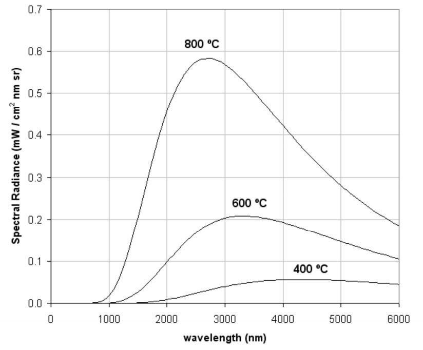 Figure 1: Spectral Radiance of a Blackbody
This behavior can be expressed mathematically in the form of Wien’s displacement law (Equation 1).
![\[ \lambda_{peak} = \frac{b}{T} \]](https://k-space.com/wp-content/ql-cache/quicklatex.com-e0827ab24e45adbbccd65b22cd724bb7_l3.png "Rendered by QuickLaTeX.com")
Equation 1: Wien’s Displacement Law
Here T is the temperature (in Kelvin), and b is a constant which equals:
![\[ \frac{hc}{4.96511\ k_B} \approx 2.8978 \times 10^6 nm \mbox {-} K \ \mathit{(See\ Appendix\ A)} \]](https://k-space.com/wp-content/ql-cache/quicklatex.com-35234e111e0c196b89105e9f3851b591_l3.png "Rendered by QuickLaTeX.com")
Note that in the temperature range of interest for typical semiconductor processing, the peak lies in the mid-IR portion of the spectrum. Thus, for the most part, BandiT spectral data comes from the short wavelength exponential tail below the peak. This often poses a challenge, as the signal intensity is relatively weak in this region.
According to Planck’s law, the spectral radiance L(λ, T) of a blackbody at a given temperature is given by:
![\[ L(\lambda,T) = \varepsilon T.F. \frac{2hc^2}{\lambda^5} \frac{1}{e^{hc/\lambda k_BT}-1}+C \]](https://k-space.com/wp-content/ql-cache/quicklatex.com-70fb5bef6be0124e2a08f8e185ab9c91_l3.png "Rendered by QuickLaTeX.com")
Equation 2: Planck’s Law
Here T is the temperature in degrees Kelvin, ε is the material’s emissivity, T.F. is a system-dependent tooling factor, and C is a constant background. A simplified version of the Planck equation can be used in the limit that hc / λkT >> 1. This is the so-called “Wien approximation” (Equation 3). This applies when the wavelength is well below the peak of the spectral radiance in Figure 1, which is typically the case at low temperatures (Wien’s displacement law states that the peak occurs at hc / λkT ≈ 4.965 – see Appendix A).
![\[ L(\lambda) \cong \varepsilon T.F. \frac{2hc^2}{\lambda^5} e^{-hc/\lambda k_BT} +C\quad (hc/\lambda k_BT >>1) \]](https://k-space.com/wp-content/ql-cache/quicklatex.com-b862218bd4a5f71407ef8e0fcf81e438_l3.png "Rendered by QuickLaTeX.com")
Equation 3: Wien’s Approximation to Planck’s Law
At a typical pyrometer wavelength of 935 nm, this approximation is quite good, introducing an error of less than 10 ppm for temperatures up to 1000ºC. At lower temperatures, the error is even further reduced. Using this approximation, and neglecting the background C, the integrated pyrometer signal over a fixed wavelength range can be represented by:
![\[ S \approx \varepsilon K e^{-c_2/\lambda T} \]](https://k-space.com/wp-content/ql-cache/quicklatex.com-b648c5ca44489bca0e92edb3a1d30caa_l3.png "Rendered by QuickLaTeX.com")
Equation 4: Pyrometer Signal Using Wien Approximation
Here c2 = hc / kB = 1.438769E+7 nm⋅K is the so-called “second radiation constant”. The constant K includes geometrical factors, viewport attenuation, and instrumental sensitivity factors (including the spectrometer integration time). K may be determined by calibrating against a blackbody at a known temperature (e.g. from a calibration source, a band edge measurement, a RHEED transition, or a Si/Al eutectic).
Once the calibration is performed, the temperature can be determined via:
![\[ \frac{1}{T} \approx \frac{1}{T_{cal}} - \frac{\lambda}{c_2} ln \left[\frac{(S^\prime - \mathit{offset}^\prime)}{(S^\prime_{cal} - \mathit{offset}^\prime) \cdot \varepsilon/\varepsilon_{cal}} \right] \]](https://k-space.com/wp-content/ql-cache/quicklatex.com-2234edc59961d35d46e0cb08b483381f_l3.png "Rendered by QuickLaTeX.com")
Equation 5: Pyrometry Equation
where the temperatures are expressed in degrees Kelvin. S′ and S′cal represent the integrated intensity, normalized to a spectrometer integration time of 1 msec. λ represents the center wavelength of the chosen band, and offset’ represents a constant background signal to be subtracted from the integrated intensity (also normalized to a spectrometer integration time of 1 msec). Note that this only requires the emissivity relative to the calibration sample. In practice, the best results are obtained by calibrating at the highest practical temperature.
This approach assumes that the tooling factor remains constant, and is therefore sensitive to viewport coatings which lead to a decrease in signal over time. Likewise, any changes in the sample emissivity over time will lead to errors.
Reference: DeWitt, D.P., Nutter, G.D., Theory and practice of Radiation Thermometry, John Wiley & Sons, New York, 1988.
BandiT Pyrometry Settings
The following settings appear in the Pyrometry dialog:
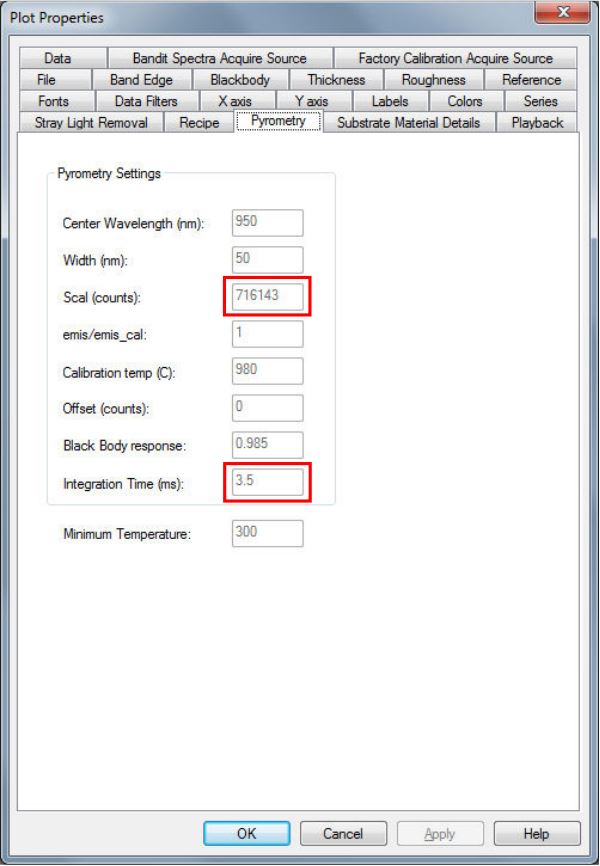 Figure 2: BandiT Pyrometry Settings
- Center Wavelength (nm): This is the center of the wavelength band over which the pyrometer signal will be summed (in this case 950 nm). This is the wavelength used in the temperature calculation (Equation 5).
- Width (nm): This represents the total width of the wavelength band over which the pyrometer signal will be summed (in this case 50 nm). For example, a value of 50 nm results in a band which extends 25 nm on either side of the center wavelength.
- Scal : This is the intensity, summed over the specified wavelength band, from the calibration procedure (S’cal = Scal divided by the spectrometer integration time in msec).
- emis/emis_cal : This is the ratio of the sample’s emissivity to that of the calibration sample (default is 1). This ratio enters into the temperature calculation via Equation 5.
- Calibration temp (C): This is the temperature in ºC at which the system was calibrated.
- Offset (counts): This constant value will be subtracted from the summed intensity via Equation 5 (the default is 0). The purpose of this is to allow the user to remove a known background signal. (offset’ = offset divided by the spectrometer integration time in msec).
- Black body response: This is intended to correct for errors introduced by both background and bandwidth effects. The latter are due to the asymmetrical nature of the Planck curve, in which the intensity is more heavily weighted toward the long wavelength end of the detector band. The size of this correction depends on the temperature and bandwidth chosen, as well as the calibration temperature. It can be represented as a linear function (Equation 6). Here T is expressed in °C. Note that the correction is typically negative (i.e. ∆T > 0 with BBR < 1), and that a value of 1 corresponds to no correction. It is therefore best determined empirically at the lowest temperature to be used. For example, using the typical range for GaAs of 935 ± 35 nm, calibrated at 1000ºC, a BBR value of 0.997 gives the correct result at 500°C.
![\[ T_{corr} = T - \Delta T, \mathit{where} \ \Delta T = (T_{cal} - T) \left( \frac{1-BBR}{BBR} \right) \]](https://k-space.com/wp-content/ql-cache/quicklatex.com-7dbf5ff7b89d749def50e0e8e502b82e_l3.png "Rendered by QuickLaTeX.com")
Equation 6: Temperature Correction
- Integration Time (msec): This is the integration time in milliseconds of the spectrum used to determine Scal during calibration.
Appendix A: Wien’s Displacement Law
The shift in the peak of the spectral radiance of a blackbody to shorter wavelengths as the temperature increases can be expressed mathematically in the form of Wien’s displacement law (Equation A-1).
Equation A-1: Wien’s Displacement Law
Here T is the temperature in Kelvin. This can be derived by first expressing the spectral radiance in terms of the dimensionless parameter x ≡ hc / λ kBT. The peak can be found by setting the first derivative with respect to x equal to zero. This leads to a non-linear equation of the form f(x) = 0, which can be solved by iterative methods. This yields:
![\[ b= \frac{hc}{4.96511\, k_B} = \frac{c_2}{4.96511} \approx 2.8978 \times 10^6 nm\mbox{-}K \ \mathit{(Figure \ A\mbox{-}1)} \]](https://k-space.com/wp-content/ql-cache/quicklatex.com-67fcd04b9da3ac181635a1002f2a89c3_l3.png "Rendered by QuickLaTeX.com")
 Figure A-1: Derivation of Wien’s Displacement Law
Appendix B: Calculating the Integrated Planck Radiance
In pyrometry, it is necessary to calculate the integrated radiance for an arbitrary wavelength range. This can be simplified by a transformation of variables to the dimensionless coordinate x (Equation B-1). The resulting definite integral can be evaluated by means of an infinite power series (Equation B-2). Fortunately, this series converges rather quickly.
![\[ \int\limits_0^\lambda L(\lambda ^\prime, T)d\lambda^\prime = \int\limits_0^\lambda \frac{2hc^2}{\lambda^{\prime 5}} \frac{d\lambda^\prime}{e^{hc/\lambda^\prime k_B T}-1} = \frac{2k^4_B T^4}{h^3c^2} \int\limits_x^\infty \frac{x^{\prime 3}}{e^{x^\prime}-1} dx^\prime, \quad where \, x \equiv \frac{hc}{\lambda k_BT} \]](https://k-space.com/wp-content/ql-cache/quicklatex.com-12651d240a18993d7e86665bfc3b39f0_l3.png "Rendered by QuickLaTeX.com")
Equation B-1: Integrated Radiance
![\[ I(x) \equiv \int\limits_x^\infty \frac{x^{\prime 3}}{e^{x^\prime}-1}dx^\prime \]](https://k-space.com/wp-content/ql-cache/quicklatex.com-93951918da5bb8520e19ca259312e755_l3.png "Rendered by QuickLaTeX.com")
![\[ \mathit{since} \; \frac{1}{e^x-1} = \sum\limits_{k=1}^\infty e^{-kx}, \quad I(x)= \sum\limits_{k=1}^\infty \int\limits_x^\infty x^{\prime 3} e^{-kx^\prime} dx^\prime \]](https://k-space.com/wp-content/ql-cache/quicklatex.com-02cad0412e060d7035b30d57b82f7b8d_l3.png "Rendered by QuickLaTeX.com")
![\[ \mathit{integrating\ by\ parts\ gives} \ I(x)= \sum\limits_{k=1}^\infty e^{-kx} \left[ \frac{x^3}{k}+\frac{3x^2}{k^2}+\frac{6x}{k^3}+\frac{6}{k^4} \right] \]](https://k-space.com/wp-content/ql-cache/quicklatex.com-1826634c43d5ef7ef472fbf35582c5cd_l3.png "Rendered by QuickLaTeX.com")
Equation B-2: Evaluation of Definite Integral via Power Series
The integrated intensity over an arbitrary range can then be calculated as the difference between two definite integrals as in Equation B-3.
![\[ \int\limits_{\lambda_{min}}^{\lambda_{max}} L(\lambda^\prime, T)d\lambda^\prime = \int\limits_{0}^{\lambda_{max}} L(\lambda^\prime, T)d\lambda^\prime - \int\limits_{0}^{\lambda_{min}} L(\lambda^\prime, T)d\lambda^\prime = \frac{2k_B^4T^4}{h^3c^2}\ \left[I(x_{max})-I(x_{min}) \right] \]](https://k-space.com/wp-content/ql-cache/quicklatex.com-7b223b80e30233f4fa0f007bff2f2c54_l3.png "Rendered by QuickLaTeX.com")
Equation B-3: Integrated Radiance over an Arbitrary Range
It is straightforward to calculate the total radiance by substituting λ=∞ (i.e. x=0) in Equation B-1. In that case, the integral in Equation B-2 reduces to a Riemann Zeta function (Equation B-4). This gives the familiar Stefan-Boltzmann law for total power emitted per unit area. Note that the additional factor of π comes from the integration over solid angle in the forward-facing hemisphere. In accordance with Lambert’s Law, the intensity is proportional to the cosine of the emission angle, measured from the surface normal (Equation B-5). Note that a surface that obeys Lambert’s Law has the same apparent radiance independent of viewing angle. Although the emitted power from a given element of surface area is reduced by the cosine of the emission angle, the size of the observed area is decreased by a corresponding amount. Therefore, the apparent radiance (i.e. power per unit projected source area per unit solid angle) is the same.
![\[ \int\limits_0^\infty L(\lambda ^\prime, T)d\lambda^\prime = \frac{2k^4_B T^4}{h^3c^2} I(0) \]](https://k-space.com/wp-content/ql-cache/quicklatex.com-6d51c562b4cd12288bd237938c8ea696_l3.png "Rendered by QuickLaTeX.com")
![\[ \mathit{with} \ I(0)= \int\limits_0^\infty \frac{x^3}{e^x-1} dx = \sum\limits_{k=1}^\infty \frac{6}{k^4} = 6 \cdot \zeta(4)=6 \cdot \frac{\pi^4}{90} = \frac{\pi^4}{15} \]](https://k-space.com/wp-content/ql-cache/quicklatex.com-2265f5dfeb68112e3b56423b3dd0d780_l3.png "Rendered by QuickLaTeX.com")
![\[ \mathit{where} \ \zeta(n) = \sum\limits_{k=1}^\infty k^{-n} \]](https://k-space.com/wp-content/ql-cache/quicklatex.com-0bcd9632f6cb57e6ebdd1ed30a410c14_l3.png "Rendered by QuickLaTeX.com")
![\[ \frac{P}{A} = \int \int\limits_0^\infty L (\lambda^\prime, T) d \lambda^\prime d\Omega = \pi \int\limits_0^\infty L (\lambda^\prime, T)d \lambda^\prime = \pi \frac{2k_B^4T^4}{h^3c^2} \frac{\pi^4}{15} = \sigma T^4 \]](https://k-space.com/wp-content/ql-cache/quicklatex.com-6262a38d6be834100627f5edd174df81_l3.png "Rendered by QuickLaTeX.com")
![\[ \mathit{where} \ \sigma \equiv \frac{2\pi^5k^4_B}{15h^3c^2} = 5.670\times 10^{-9} mW \cdot cm^{-2} \cdot K^{-4} \]](https://k-space.com/wp-content/ql-cache/quicklatex.com-f44b63ec1f674d8e0299cdcf89ddf069_l3.png "Rendered by QuickLaTeX.com")
Equation B-4: Derivation of the Stefan-Boltzmann Law
![\[ d\Omega = \sin \theta d \theta d \varphi, \ 0 \leq \theta \leq \pi/2, 0\leq \varphi \leq 2\pi \]](https://k-space.com/wp-content/ql-cache/quicklatex.com-1f567a2090b862f4b05195ad2fd6accc_l3.png "Rendered by QuickLaTeX.com")
![\[ \int \cos \theta d \Omega = \int\limits^{2\pi}_0 d \varphi \int\limits^\theta_0 \cos \theta^\prime \sin \theta^\prime d \theta^\prime = \pi (1-\cos^2 \theta) \]](https://k-space.com/wp-content/ql-cache/quicklatex.com-78d71ddb2da24cb7725a739be57e0a03_l3.png "Rendered by QuickLaTeX.com")
![\[ \mathit{for} \ \theta = \pi/2, \int \cos \theta d\Omega = \pi \]](https://k-space.com/wp-content/ql-cache/quicklatex.com-5964a46fe7e9ca9d58b67e298f10083b_l3.png "Rendered by QuickLaTeX.com")
Equation B-5: Lambert’s Law Angular Dependence